how to draw 3d vector diagrams

março 09, 2022 Postar um comentário

folds2d.tumblr.com

f03370000E4D3

The goal

During last few days I've made several attempts to create and visualize 2D vector fields. In the following article you lot tin read nigh this concept with several examples and code in Processing.

There are many cute fine art/code based on vector field visualization around the cyberspace. By and large based on dissonance function. Check them out before you first:

Visualizer by p5art
Furfrolic past Holger Lippmann
My own 2 sketches drawing_generative and threadraw
Few examples on OpenProcessing site: i, 2, 3, 4

What is the vector field?

Vector field (in our example) is just a $\mathbf{R}^{2}$ to $\mathbf{R}^{2}$ function exatly the same as variation described in my previous post about Folds.

Why vector? Because you tin treat a pair of $(x',y')$ every bit vector $\vec{v} = \begin{bmatrix}x'\\ y'\end{bmatrix}$ for each bespeak from 2d plane. This way y'all get field of vectors.

Vector fields can be visualised in the following way

How to get the vector field

The master goal, in this article, is to research various ways to create vector fields. There ii cases.

We can operate on functions which returns pair of values like variations. In this case such part defines vector field itself. Nosotros can use too some vector operations (like substraction, sum, etc…) to get new functions.

The second pick is to get single float number $n$ like from noise(), dist() between points or dot production of vectors, etc. And convert this number into vector.

Drawing method

The method is quite elementary.

Create points from $[-3,3]$ floating bespeak range
Describe them
For each of the point calculate relating vector from the vector field
Scale information technology and add to the bespeak coordinates
Repeat two-four

Step 4 is primal here. We move our points along vectors. Trace lines build the resulting image.

The full general menses for constructing vector field follows this scheme:

$p=(x,y)\mapsto [multiple operations]\mapsto \vec{v}$

Note: I assume that on every step I can multiply function variables or returned values past any number.

Here is code stub for my experiments

// dynamic list with our points, PVector holds position ArrayList<PVector> points = new ArrayList<PVector>();  // colors used for points color[] pal = {   color(0, 91, 197),   color(0, 180, 252),   color(23, 249, 255),   colour(223, 147, 0),   color(248, 190, 0) };  // global configuration float vector_scale = 0.01; // vector scaling factor, we desire small steps float time = 0; // time passes by  void setup() {   size(800, 800);   strokeWeight(0.66);   background(0, v, 25);   noFill();   smooth(viii);    // noiseSeed(1111); // sometimes nosotros select 1 racket field    // create points from [-three,three] range   for (bladder ten=-3; x<=3; 10+=0.07) {     for (float y=-3; y<=three; y+=0.07) {       // create indicate slightly distorted       PVector 5 = new PVector(10+randomGaussian()*0.003, y+randomGaussian()*0.003);       points.add(5);     }   } }  void draw() {   int point_idx = 0; // point index   for (PVector p : points) {     // map floating betoken coordinates to screen coordinates     float twenty = map(p.x, -6.5, 6.5, 0, width);     float yy = map(p.y, -six.five, 6.five, 0, peak);      // select colour from palette (index based on racket)     int cn = (int)(100*pal.length*noise(point_idx))%pal.length;     stroke(pal[cn], 15);     point(20, yy); //draw      // placeholder for vector field calculations      // 5 is vector from the field     PVector 5 = new PVector(0, 0);      p.x += vector_scale * v.x;     p.y += vector_scale * v.y;      // go to the next betoken     point_idx++;   }   time += 0.001; }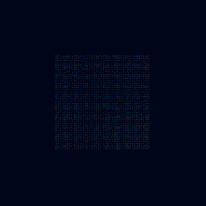

f014700009714

When I change my field vector to be abiding ane (unlike than 0), my points kickoff motility.

PVector v = new PVector(0.ane, 0.1);

f056900004085

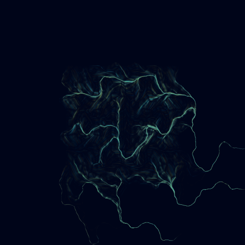
Perlin noise

Allow's brainstorm with perlin noise in few configurations. I'm going to alter just marked lines from the code stub.

Variant 1

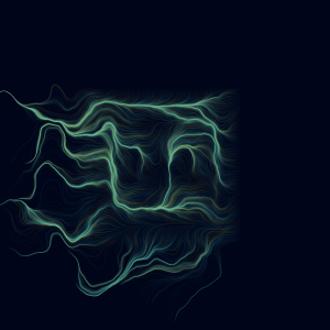
noise(x,y) part in processing returns value from 0 to 1 (really implementation used in Processing has some issues and real value is oftentimes in range from 0.2 to 0.8). I will care for resulted value every bit an angle in polar coordinates and employ sin()/cos() functions to convert it to cartesian ones. To properly practise this I have to calibration it up to range $[0,2\pi ]$ or $[-\pi, \pi ]$ or fifty-fifty more. I show few variants here.

// placeholder for vector field calculations float northward = TWO_PI * noise(p.x,p.y); PVector v = new PVector(cos(n),sin(due north));

f043800005B6A

Variant 2

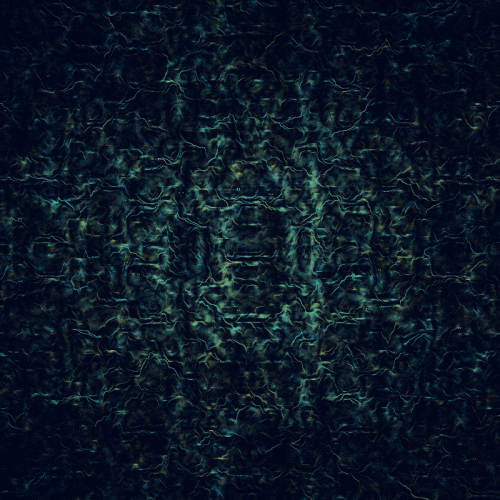
Let's check what happens when I multiply racket by ten, 100, 300 or fifty-fifty 1000. Noise is at present scaled to range $[-1.1]$ (it is more usable range in further examples).

float n = 10 * map(dissonance(p.ten/5,p.y/v),0,ane,-ane,1); // 100, 300 or 1000 PVector v = new PVector(cos(n),sin(n));

1000

Variant 3

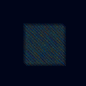
2 of above variants were using archetype method. At present I get rid of polar->cartesian conversion and I'thou going to treat returned value from noise() equally cartesian coordinates. Angle of the vector is the same for whole field and only length of vector is changed. This leads to some interesting patterns. Experiment with scaling input coordinates and $n$

float n = 5*map(noise(p.10,p.y),0,1,-1,one); PVector v = new PVector(n,due north);

Parametric curves

Let's apply parametric curves to catechumen dissonance() result into vector. The large list of them is defined in Wolfram Blastoff or named here. Parametric curve (or plane bend) is a function $\mathbf{R}\rightarrow\mathbf{R}^2$ . Click section name to see plot of the curve.

Astroid

// placeholder for vector field calculations bladder n = v*map(dissonance(p.ten,p.y),0,1,-ane,1); // and two  bladder sinn = sin(n); float cosn = cos(north);  float xt = sq(sinn)*sinn; bladder yt = sq(cosn)*cosn;  PVector v = new PVector(xt,yt);

Results for noise calibration ii and 5

Cissoid of Diocles

// placeholder for vector field calculations float n = 3*map(noise(p.x,p.y),0,one,-1,ane);  bladder sinn2 = 2*sq(sin(northward));  float xt = sinn2; bladder yt = sinn2*tan(due north);  PVector v = new PVector(xt,yt);

f146100000B07

Kampyle of Eudoxus

// placeholder for vector field calculations float n = 6*map(noise(p.x,p.y),0,1,-one,1);  bladder sec = 1/sin(n);  float xt = sec; float yt = tan(n)*sec;   PVector five = new PVector(xt,yt);

f08490000B8A6

Rectangular Hyperbola

// placeholder for vector field calculations float north = 10*map(dissonance(p.10*2,p.y*2),0,1,-1,1);  float xt = ane/sin(northward); float yt = tan(n);   PVector five = new PVector(xt,yt);

f123200005CCF

Superformula

// placeholder for vector field calculations float n = five*map(dissonance(p.ten,p.y),0,one,-1,one);  float a = i; float b = 1; bladder m = half-dozen; bladder n1 = 1; float n2 = 7; float n3 = 8;  bladder f1 = pow(abs(cos(chiliad*due north/4)/a),n2); bladder f2 = pow(abs(sin(m*due north/4)/b),n3); float fr = pow(f1+f2,-1/n1);  float xt = cos(north)*fr; bladder yt = sin(n)*fr;  PVector five = new PVector(xt,yt);

f034900000FCF

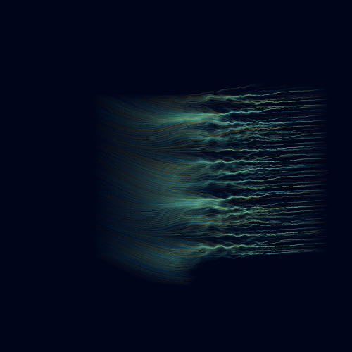
Noise and curves combined

At present I'm going to play with some combinations of above curves and make multiple passes through noise().

Allow's put all curves into functions (paste following code to the end of the script):

PVector circumvolve(float northward) { // polar to cartesian coordinates   return new PVector(cos(n), sin(n)); }  PVector astroid(float northward) {   float sinn = sin(northward);   bladder cosn = cos(n);    bladder xt = sq(sinn)*sinn;   float yt = sq(cosn)*cosn;    return new PVector(xt, yt); }  PVector cissoid(bladder northward) {   float sinn2 = 2*sq(sin(northward));    float xt = sinn2;   bladder yt = sinn2*tan(n);    render new PVector(xt, yt); }  PVector kampyle(float north) {   bladder sec = i/sin(n);    float xt = sec;   float yt = tan(n)*sec;    return new PVector(xt, yt); }  PVector rect_hyperbola(float n) {   float sec = ane/sin(n);    float xt = 1/sin(northward);   bladder yt = tan(n);    return new PVector(xt, yt); }  final static float superformula_a = one; concluding static float superformula_b = one; final static float superformula_m = 6; final static float superformula_n1 = i; final static float superformula_n2 = vii; final static bladder superformula_n3 = eight; PVector superformula(float northward) {   bladder f1 = pow(abs(cos(superformula_m*northward/4)/superformula_a), superformula_n2);   float f2 = pw(abs(sin(superformula_m*northward/four)/superformula_b), superformula_n3);   float fr = prisoner of war(f1+f2, -ane/superformula_n1);    float xt = cos(north)*fr;   float yt = sin(n)*fr;    render new PVector(xt, yt); }

Variant 1 – p5art

Code based on p5art spider web app noisePainting

$point\rightarrow noise\rightarrow noise\rightarrow noise\rightarrow vector$

// placeholder for vector field calculations float n1 = 10*noise(one+p.x/twenty, i+p.y/20); // shift input to avert symetry float n2 = 5*dissonance(n1, n1); bladder n3 = 325*map(noise(n2, n2), 0, 1, -1, ane); // 25,325  PVector v = circumvolve(n3);

Variant two

$point\rightarrow noise\rightarrow curves\rightarrow noise\rightarrow noise\rightarrow circle\rightarrow vector$

// placeholder for vector field calculations float n1 = 15*map(racket(1+p.x/xx, one+p.y/twenty),0,1,-one,ane);  PVector v1 = cissoid(n1); PVector v2 = astroid(n1);  float n2a = 5*dissonance(v1.x,v2.y); float n2b = five*noise(v2.x,v1.y);  bladder n3 = 10*map(noise(n2a, n2b/3), 0, 1, -1, one);  PVector v = circle(n3);

f071000004C6F

Variant 3

$point\rightarrow noise\rightarrow curves\rightarrow noises\rightarrow vector$

// placeholder for vector field calculations float n1 = 15*map(noise(1+p.x/10, ane+p.y/10),0,1,-ane,i);  PVector v1 = rect_hyperbola(n1); PVector v2 = astroid(n1);  float n2a = 2*map(racket(v1.x,v1.y),0,one,-ane,1); float n2b = 2*map(noise(v2.10,v2.y),0,one,-1,i);  PVector v = new PVector(n2a,n2b);

f056400001094

Variant 4

$point\rightarrow curves\rightarrow noises\rightarrow circle\rightarrow vector$

// placeholder for vector field calculations PVector v1 = kampyle(p.x); PVector v2 = superformula(p.y);  float n2a = 3*map(noise(v1.x,v1.y),0,1,-1,i); float n2b = 3*map(noise(v2.x,v2.y),0,1,-1,i);  PVector 5 = new PVector(cos(n2a),sin(n2b));

f04470000695F

Variant 5

$point\rightarrow noises\rightarrow curves\rightarrow noises\rightarrow circle\rightarrow vector$

// placeholder for vector field calculations float n1a = 3*map(noise(p.x,p.y),0,1,-ane,1); float n1b = 3*map(racket(p.y,p.x),0,1,-i,1);  PVector v1 = rect_hyperbola(n1a); PVector v2 = astroid(n1b);  float n2a = 3*map(noise(v1.x,v1.y),0,1,-ane,one); float n2b = three*map(dissonance(v2.x,v2.y),0,1,-one,ane);  PVector five = new PVector(cos(n2a),sin(n2b));

f04750000BD8E

Variant half dozen – comparison

Hither I desire to compare dissimilar curves using the same method. I change marked lines into pair of curves defined above. I've putnoiseSeed(1111); in setup() to have the same racket construction. Check image description to encounter what curves were used.

$point\rightarrow curves\rightarrow subtract\rightarrow vector$

// placeholder for vector field calculations float n1a = 15*map(noise(p.10/10,p.y/10),0,1,-ane,1); float n1b = 15*map(noise(p.y/10,p.x/10),0,one,-ane,1);  PVector v1 = superformula(n1a); PVector v2 = circumvolve(n1b);  PVector diff = PVector.sub(v2,v1); diff.mult(0.3);  PVector v = new PVector(diff.ten,unequal.y);

kampyle, rect_hyperbola

kampyle, cissoid

astroid, kampyle

astroid, cissoid

circle, cissoid

rect_hyperbola, superformula

superformula, circle

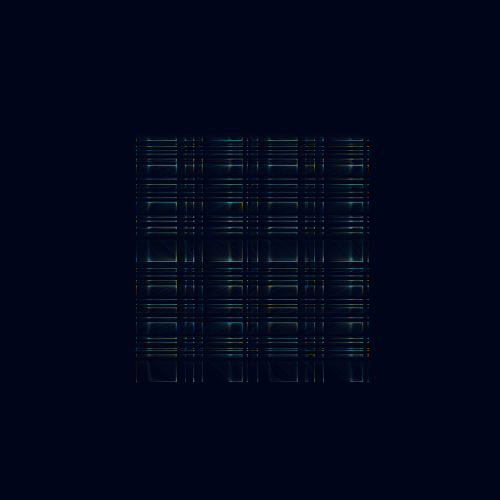
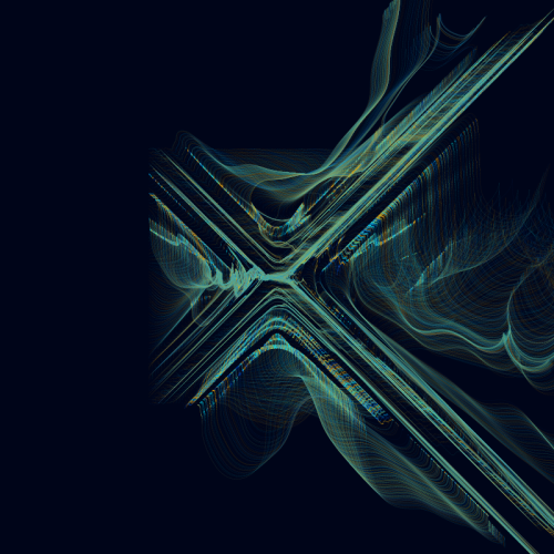
Time

Now permit's introduce time. An external variable which is incremented every frame with some small value. It can be used to slightly alter dissonance field during rendrering or can be used every bit a scale cistron.

Let's compare the same vector field without time and time used as tertiary racket parameter.

          // placeholder for vector field calculations  bladder n1a = 3*map(noise(p.x/2,p.y/2),0,1,-1,1);  float n1b = 3*map(noise(p.y/2,p.ten/two),0,i,-i,i);  float nn = 6*map(noise(n1a,n1b),0,1,-i,1);   PVector v = circle(nn);

f041800008831

And now I add time as a third parameter to noise function. This way our vector field changes when time passes.

          // placeholder for vector field calculations bladder n1a = 3*map(noise(p.ten/2,p.y/2,time),0,1,-1,1); float n1b = 3*map(noise(p.y/ii,p.x/2,time),0,ane,-ane,i); float nn = half-dozen*map(noise(n1a,n1b,time),0,ane,-1,1);  PVector v = circle(nn);

f051900001798

At present time is used as a scaling factor.

// placeholder for vector field calculations float n1a = 3*map(racket(p.ten/2,p.y/2),0,ane,-ane,1); bladder n1b = three*map(racket(p.y/2,p.x/two),0,1,-1,1);  bladder nn = time*x*6*map(dissonance(n1a,n1b),0,1,-1,1);  PVector v = circle(nn);

f089600004548

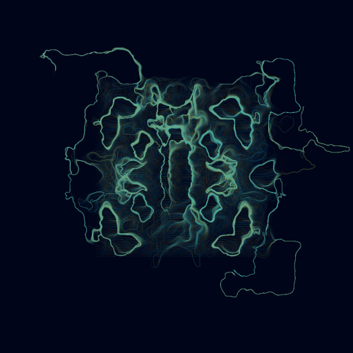
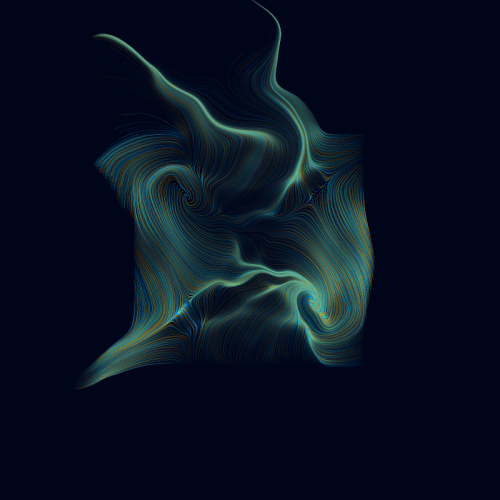
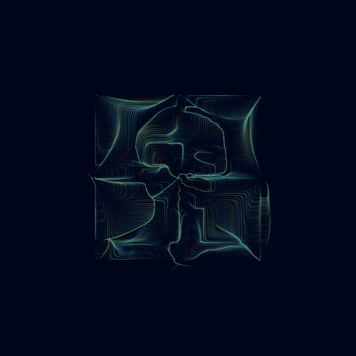
Variations

Now let's innovate variations (run across previous mail about Folds) as a vector field definition.

Re-create beneath code to the end of your sketch. Information technology includes function definiotions used in this and side by side capacity.

PVector sinusoidal(PVector v, float amount) {   render new PVector(amount * sin(v.x), corporeality * sin(v.y)); }  PVector waves2(PVector p, float weight) {   float x = weight * (p.x + 0.9 * sin(p.y * 4));   float y = weight * (p.y + 0.five * sin(p.x * 5.555));   return new PVector(x, y); }  PVector polar(PVector p, float weight) {   float r = p.magazine();   bladder theta = atan2(p.x, p.y);   float x = theta / PI;   float y = r - 2.0;   return new PVector(weight * x, weight * y); }  PVector swirl(PVector p, bladder weight) {   bladder r2 = sq(p.x)+sq(p.y);   float sinr = sin(r2);   float cosr = cos(r2);   bladder newX = 0.eight * (sinr * p.ten - cosr * p.y);   float newY = 0.eight * (cosr * p.y + sinr * p.y);   return new PVector(weight * newX, weight * newY); }  PVector hyperbolic(PVector v, float amount) {   float r = v.mag() + 1.0e-10;   float theta = atan2(v.x, 5.y);   bladder x = amount * sin(theta) / r;   float y = amount * cos(theta) * r;   return new PVector(x, y); }  PVector ability(PVector p, float weight) {   bladder theta = atan2(p.y, p.x);   bladder sinr = sin(theta);   float cosr = cos(theta);   float pw = weight * pow(p.mag(), sinr);   return new PVector(prisoner of war * cosr, pow * sinr); }  PVector cosine(PVector p, float weight) {   float pix = p.x * PI;   float x = weight * 0.8 * cos(pix) * cosh(p.y);   bladder y = -weight * 0.8 * sin(pix) * sinh(p.y);   return new PVector(x, y); }  PVector cross(PVector p, float weight) {   float r = sqrt(1.0 / (sq(sq(p.10)-sq(p.y)))+ane.0e-10);   return new PVector(weight * 0.8 * p.x * r, weight * 0.8 * p.y * r); }  PVector vexp(PVector p, float weight) {   float r = weight * exp(p.x);   return new PVector(r * cos(p.y), r * sin(p.y)); }  // parametrization P={pdj_a,pdj_b,pdj_c,pdj_d} float pdj_a = 0.one; float pdj_b = 1.9; float pdj_c = -0.8; float pdj_d = -ane.2; PVector pdj(PVector 5, float amount) {   return new PVector( amount * (sin(pdj_a * v.y) - cos(pdj_b * 5.x)),   amount * (sin(pdj_c * v.10) - cos(pdj_d * v.y))); }  final bladder cosh(bladder x) { return 0.v * (exp(10) + exp(-10));} final float sinh(float x) { return 0.five * (exp(10) - exp(-x));}

Permit's see how individual variations look equally vector fields. Sometimes I had to adjust scaling factor to keep points on the screen.

// placeholder for vector field calculations PVector v = sinusoidal(p,1); v.mult(1); // different values for unlike functions

All together

Let'south sumarize what functions we have now defined.

All to a higher place operations can exist used to generate vector field (or simply transform 2d indicate to another second betoken).

I will play with to a higher place transformations in post-obit examples. Information technology's a record of experiments.

Variant one

$point\rightarrow variations\rightarrow circle\rightarrow vector$

// placeholder for vector field calculations float n1 = 5*map(noise(p.ten/5,p.y/five),0,1,-1,1);  PVector v1 = rect_hyperbola(n1); PVector v2 = swirl(v1,1);  PVector five = new PVector(cos(v2.x),sin(v2.y));

f049300008710

Variant 2

$point\rightarrow noises\rightarrow variations\rightarrow subtraction\rightarrow variation\rightarrow vector$

// placeholder for vector field calculations bladder n1 = 5*map(noise(p.x/5,p.y/5),0,ane,-1,one); bladder n2 = 5*map(noise(p.y/five,p.x/5),0,1,-1,1);  PVector v1 = vexp(new PVector(n1,n2),one); PVector v2 = swirl(new PVector(n2,n1),1);  PVector v3 = PVector.sub(v2,v1);  PVector v4 = waves2(v1,1); v4.mult(0.8);  PVector v = new PVector(v4.ten,v4.y);

f04190000D54D

Variant 3

$point\rightarrow variation\rightarrow noises\rightarrow variation\rightarrow vector$

// placeholder for vector field calculations PVector v1 = vexp(p,1);  float n1 = map(dissonance(v1.10,v1.y,fourth dimension),0,1,-1,one); bladder n2 = map(noise(v1.y,v1.x,-time),0,ane,-ane,1);  PVector v2 = vexp(new PVector(n1,n2),1);  PVector v = new PVector(v2.ten,v2.y);

f028600002221

Variant iv

$point\rightarrow variation\rightarrow noise\rightarrow curve\rightarrow normalization\rightarrow vector$

// placeholder for vector field calculations PVector v1 = polar(cross(p,ane),1);  float n1 = fifteen*map(dissonance(v1.10,v1.y,time),0,1,-1,ane); PVector v2 = cissoid(n1); v2.normalize();  PVector v = new PVector(v2.x,v2.y);

f08680000EA5D

Variant 5

$point\rightarrow variation\rightarrow noises\rightarrow variation\rightarrow angle\rightarrow variation\rightarrow circle\rightarrow vector$

// placeholder for vector field calculations PVector v1 = power(p,1);  float n1 = v*map(dissonance(v1.x,v1.y,fourth dimension),0,ane,-1,one); float n2 = 5*map(noise(p.10/iii,p.y/3,-time),0,one,-1,ane);  PVector v2 = cosine(new PVector(n1,n2),1);  bladder a1 = PVector.angleBetween(v1,v2);  PVector v3 = superformula(a1); v3.mult(3);  PVector v = new PVector(cos(v3.x),sin(v3.y));

f04770000F923

Variant 6

$point\rightarrow variation\rightarrow subtraction\rightarrow angles\rightarrow combination \rightarrow circle\rightarrow vector$

// placeholder for vector field calculations PVector v1 = waves2(p,1); PVector v2 = PVector.sub(v1,p);  float n1 = viii*dissonance(time)*atan2(v1.y,v1.x); float n2 = eight*dissonance(time+0.v)*atan2(v2.y,v2.ten);  PVector five = new PVector(cos(v2.x*n1),sin(v1.y+n2));

f035200007633

Variant seven

$point\rightarrow variation\rightarrow subtraction\rightarrow noises\rightarrow angles\rightarrow curves\rightarrow variations\rightarrow subtraction\rightarrow variation\rightarrow angle\rightarrow combination\rightarrow circle\rightarrow vector$

// placeholder for vector field calculations PVector v1 = swirl(p,1); v1.mult(0.five); PVector v2 = PVector.sub(v1,p);  float nv1 = noise(v1.ten,v1.y,time); float nv2 = noise(v2.10,v2.y,-fourth dimension);  float n1 = (atan2(v1.y,v1.10)+nv2); bladder n2 = (atan2(v2.y,v2.10)+nv1);  PVector v3 = superformula(n1); PVector v4 = rect_hyperbola(n2);  PVector tv3 = waves2(v3,1); PVector tv4 = sinusoidal(v4,1);  PVector v5 = PVector.sub(tv4,tv3);  PVector v6 = pdj(v5,1);  bladder an = PVector.angleBetween(v6,new PVector(n1,n2));  PVector five = new PVector(cos(v2.x+sin(an)),sin(v6.y-cos(an))); v.mult(1+time*xl);

f040300002B89

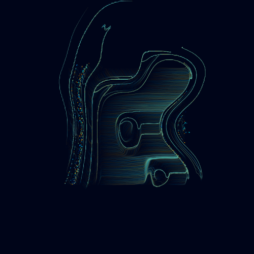
Image

The concluding part is virtually using aqueduct information from an image as a vector field. I wrote two sketches some time ago which are based on vector field concept.

Drawing generative

res_75948_natalie

Threadraw

res_4BC7E81C_natalie

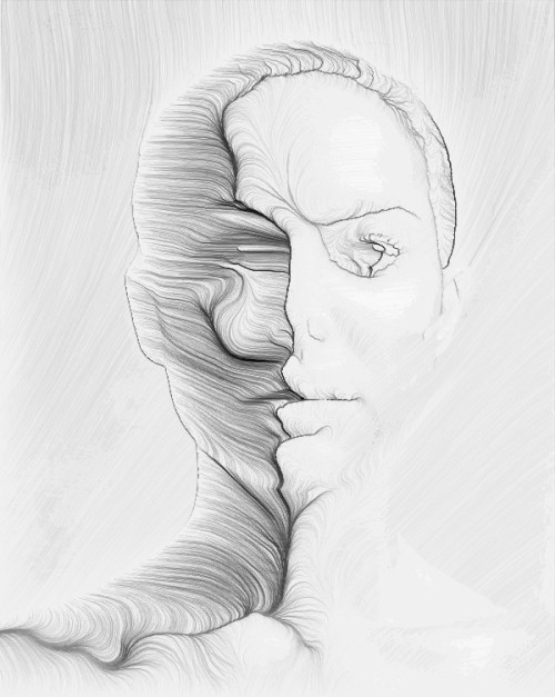
How to apply image data

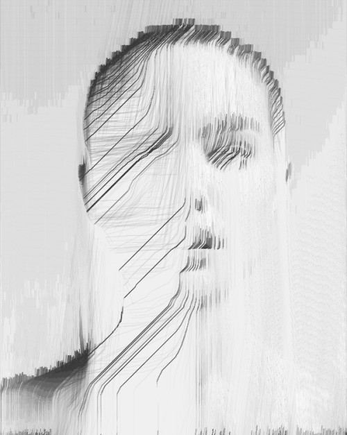
First load your epitome at the beginning of the sketch

img = loadImage("natalie.jpg"); // PImage img; must be declared globally

And so use epitome data following way

// placeholder for vector field calculations PVector v1 = sinusoidal(p,1);  int img_x = (int)map(p.x,-3,three,0,img.width); int img_y = (int)map(p.y,-three,three,0,img.height);  float b = brightness( img.get(img_x,img_y) )/255.0; PVector br = circle(b);  float a = five*PVector.angleBetween(br,v1);  PVector v = astroid(a);

f015500000067

Appendix

This concept is taken from zach lieberman and Keith Peters who explored painting by non-intersecting segments. This thought tin be used on vector fields too. Hither are two examples.

See the code HERE.

The end

Questions? generateme.weblog@gmail.com or Follow @generateme_blog

boweharbeadven.blogspot.com

Source: https://generateme.wordpress.com/2016/04/24/drawing-vector-field/

how to draw 3d vector diagrams

folds2d.tumblr.com

The goal

What is the vector field?

How to get the vector field

Drawing method

Perlin noise

Variant 1

Variant 2

Variant 3

Parametric curves

Astroid

Cissoid of Diocles

Kampyle of Eudoxus

Rectangular Hyperbola

Superformula

Noise and curves combined

Variant 1 – p5art

Variant two

Variant 3

Variant 4

Variant 5

Variant half dozen – comparison

Time

Variations

All together

Variant one

Variant 2

Variant 3

Variant iv

Variant 5

Variant 6

Variant seven

Image

Drawing generative

Threadraw

How to apply image data

Appendix

The end

Postar um comentário for "how to draw 3d vector diagrams"